Silent Parties: A Cluster Analysis of Voting Behavior in the European Parliament


Welcome to this interactive application, designed to explore and analyze the clustering of voting behaviors within the European Parliament. This tool provides insights into how Members of the European Parliament (MEPs) form latent voting blocs based on their voting patterns. Using advanced dimensionality reduction techniques like UMAP, MCA, and DW-NOMINATE, as well as clustering methods such as K-Means, PAM, and HDBSCAN, this application allows you to investigate the ideological alignments and coalitions that emerge within the EU legislative body. Don't worry if you're new to these techniques! This app provides an intuitive interface to guide you through each step, offering visuals and interpretations to help you understand the complex relationships between MEPs.


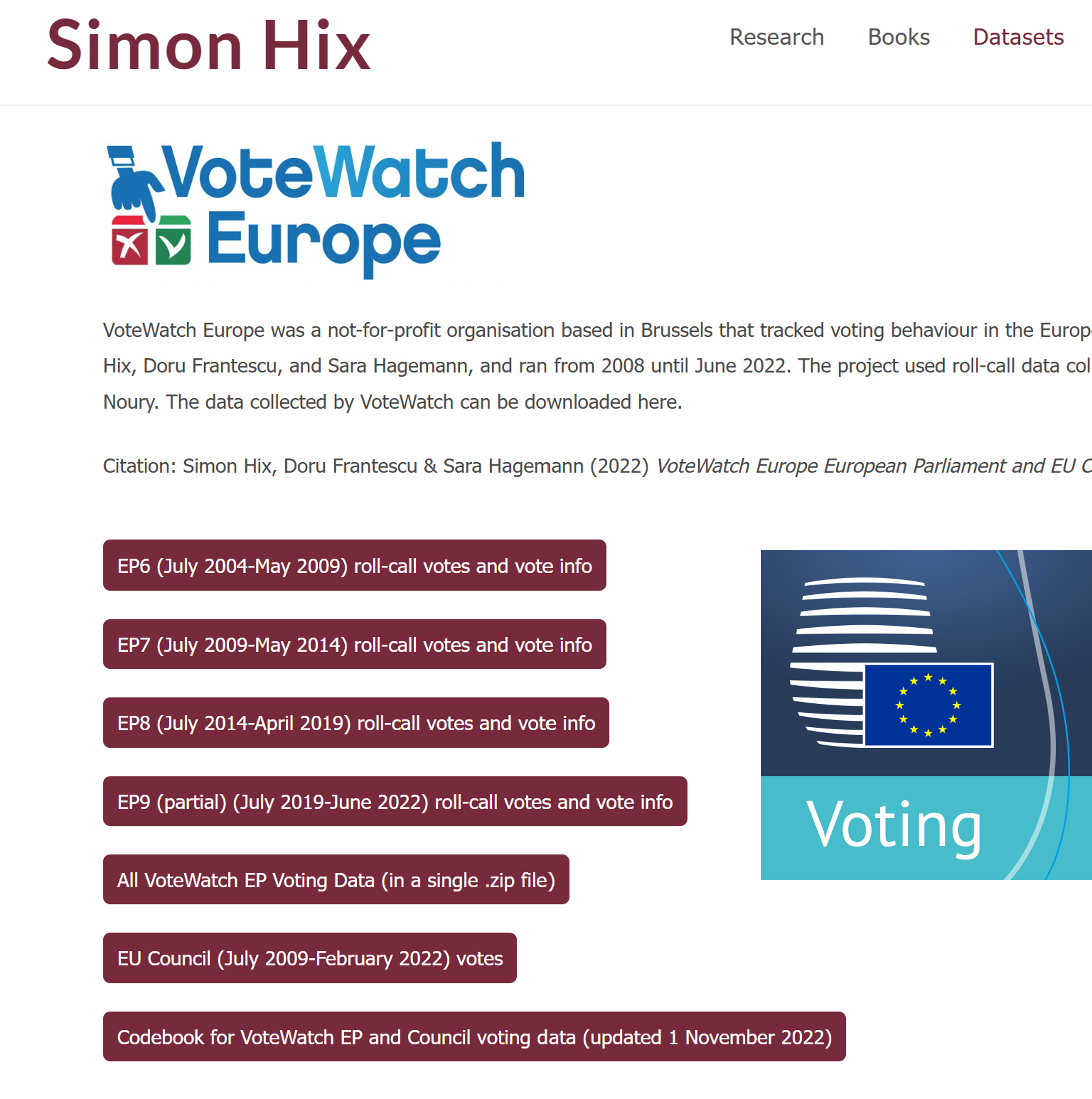
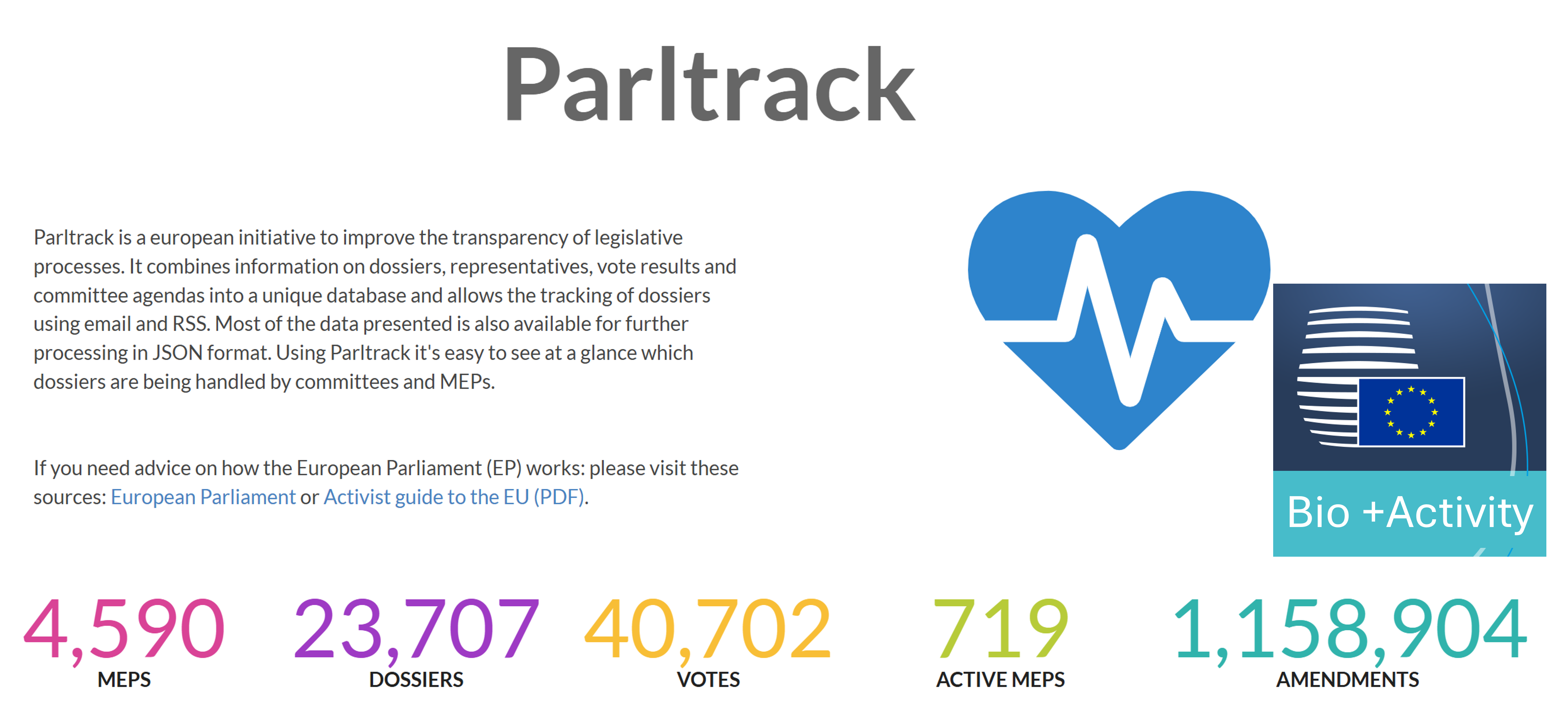
The data used in this application are publicly accessible through the VoteWatch Europe and PollTrack.eu databases. These data sources contain voting records and biographical information for MEPs, covering multiple EU legislative sessions from 2004 to 2022. By leveraging this comprehensive dataset, you can gain insights into how political groups, alliances, and individual MEPs align on critical issues across different policy areas, including economics, foreign policy, social issues, and more.


For more information please check the European Parliament page clicking
Here


How to Use this App


How This Project Came to Be


This application allows you to explore the complexities of MEP voting behavior through various analytical lenses. My hope is that it reveals some of the nuances within the European Parliament and inspires further exploration.

Inspiration

The idea to analyze voting behavior in the European Parliament started with a simple question: Are there hidden patterns in the way MEPs vote?

Data Collection

Using publicly available data on MEPs' voting records, I gathered detailed datasets spanning multiple legislative periods.

Data Processing

Data cleaning, filtering, and encoding helped prepare the dataset for deeper analysis, ensuring accuracy in every step.

Exploratory Analysis

With visualizations and statistical summaries, I began uncovering initial patterns and trends in the voting data.

Dimensionality Reduction

Using UMAP, MCA, and DW-NOMINATE, I transformed high-dimensional voting data into a compact format for clustering.

Clustering

Applying K-Means, PAM, and HDBSCAN, I identified clusters representing potential political groups or alliances.

Validation

Metrics like silhouette score and stability analysis validated the clusters' reliability, ensuring meaningful insights.


Submitted in partial fulfillment of the requirements
for the degree of Master of Science

Developed by
John F. Brüne

Introduction - Defining the Problem


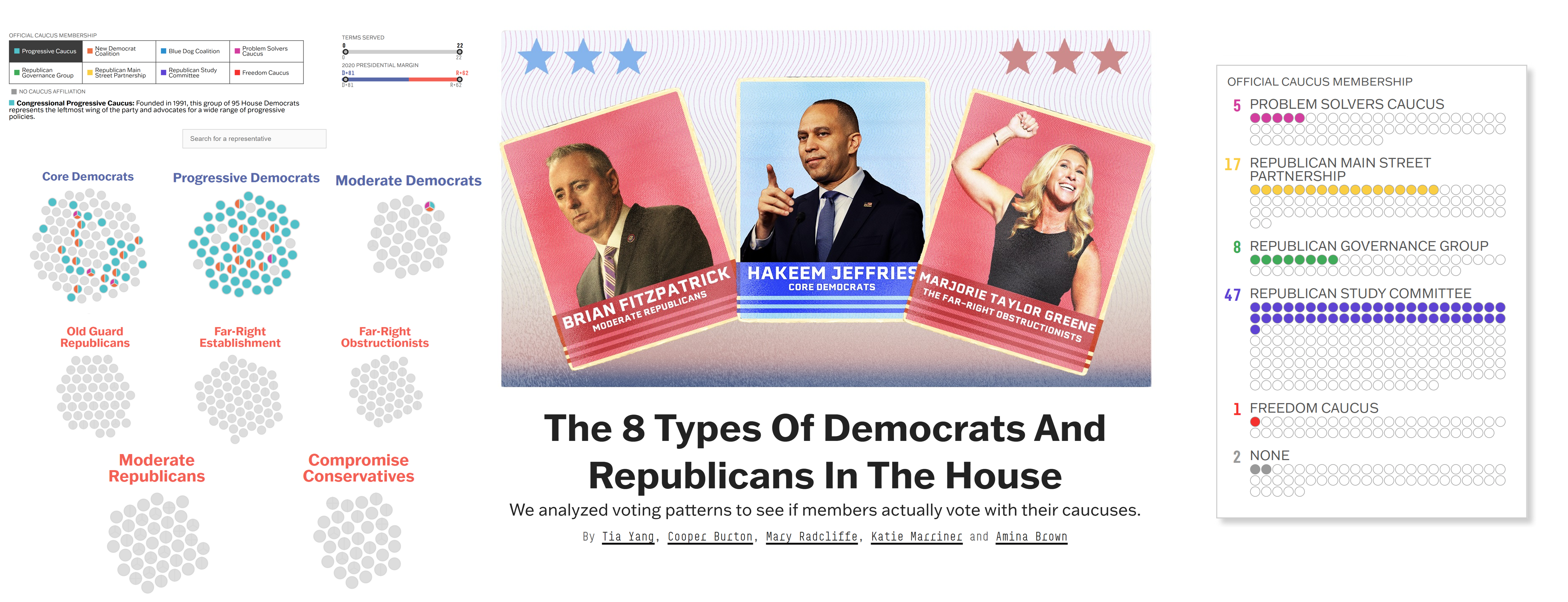
In May 2024 the U.S. website FiveThirtyEight conducted an analysis to explore patterns in the voting behavior of U.S. House members. They used the K-Means clustering algorithm to categorize representatives into 8 distinct clusters based on their voting records. However, this example serves as a reminder of the challenges of clustering unlabelled data: there is no single 'correct' number of clusters. Depending on how we choose to analyze the data, we could find 4, 8, or even 10 clusters, without a definitive answer as to which is most accurate.

In the following tabs, this study will turn to similar data from the European Parliament, aiming to explore the same clustering challenge and investigate how representatives form latent voting blocs based on their behavior.


Graphical tests


The K-Means algorithm aims to minimize the following objective function:

$$ \text{argmin} \sum_{i=1}^{k} \sum_{x_j \in C_i} || x_j - \mu_i ||^2 $$

Here, \(k\) represents the number of clusters, \(x_j\) are the data points (voting records), and \(\mu_i\) represents the centroid of each cluster \(C_i\). The algorithm iteratively adjusts these centroids to minimize within-cluster variance, but the selection of \(k\) remains subjective. The clustering of unlabelled data is inherently flexible — meaning that one dataset could yield different numbers of clusters depending on interpretation and goals.


Analytical tests


Remember, the interpretation of each metric is important in determining clustering quality.


Data Preparation


"In God we trust. All others must bring data."

~ W. Edwards Deming


Data preparation is a critical phase in any analysis, ensuring that the data is clean, standardized, and ready for modeling. In this section, we outline the key steps we took to prepare the voting data from the European Parliament for clustering. These steps are designed to create a robust dataset that accurately represents the voting patterns and ideological positions of the Members of the European Parliament (MEPs).


1. Data Collecting

The dataset was carefully collected from publicly available voting records of the European Parliament. Each record contains information on votes cast by Members of the European Parliament (MEPs) across various issues, allowing us to analyze their political alignment and engagement. This initial step ensures we have a comprehensive dataset for meaningful analysis.


2. Data Cleaning

To ensure data quality, we applied a complete case analysis approach, removing any records with missing values. By doing so, we can rely on each observation in the dataset as a full representation of each MEP's voting behavior, leading to more accurate and reliable clustering results.


3. Feature Engineering

In this step, we used our raw data to create more meaningful variables.


4. Data Transformation

To prepare the dataset for clustering, we standardized each feature, setting the mean to zero and the standard deviation to one. This transformation ensures that all variables contribute equally, enhancing the clustering algorithm's ability to detect patterns across different dimensions of voting behavior.


Merged Data Preview

The merged data preview will appear here after merging.


Data Preview


Feature Engineering Results

Feature Explanation
Distribution Plot

Visualize the distribution of the newly engineered features below to ensure they are properly calculated.


Select a variable from the sidebar to see its distribution before and after transformation.

Transformations can reveal hidden patterns or make data more suitable for modeling. Here’s an example visualization comparing the original and transformed data distributions.


Original Distribution
Transformed Distribution

Final Dataset Summary


Exploratory Analysis

In this step, we delve into the key patterns and relationships within the voting behavior data of the European Parliament. Exploratory analysis is essential for understanding how MEPs (Members of the European Parliament) align on different issues, which factions tend to vote together, and how individual MEP characteristics might correlate with voting behavior. This preliminary step will help us determine relevant variables for clustering and ultimately guide our grouping decisions.

Use the options below to select variables of interest and generate visualizations that reveal underlying structures in the data. For instance, you might explore how different political groups or countries align on specific voting topics, or examine the attendance and activity levels of MEPs. Additionally, interactive maps and summary tables are provided to give you a comprehensive view of the data.


Exploratory Plots and Statistics

The exploratory plots and statistics below provide insights into the distribution and relationships within the selected variables. Use these visualizations to identify notable voting patterns, similarities, and differences among MEPs. You may find that certain groups consistently align on votes, while others show greater variability.


Please finish the Data Preparation first.

Please finish the Data Preparation first.

Interpretation of Box Plot

The box plot visualizes the distribution of the selected variable(s) across different categories, such as political groups (EPGs) or countries. Each box represents the spread of data for one category, showing the median, interquartile range, and potential outliers. This helps in identifying which groups have more homogeneous voting behavior or attendance levels and which ones display greater variation.

For instance, a narrow box with minimal outliers indicates that a group's members tend to behave similarly on the selected measure, while a wider box or multiple outliers may suggest diverse voting patterns within that group.


Country Map

The map visualizes the selected measure (such as attendance or voting alignment) by country. This can help you observe geographical patterns in the data, such as higher engagement in certain regions or countries with MEPs who tend to vote together.


Summary Table

This table provides a summary of the selected variable(s) for each political group or country. Use this table to identify differences across groups, such as variations in average attendance scores or voting alignments. Sorting by mean can be useful for highlighting key trends and outliers.


Parliament View


Please finish the Data Preparation first.

Dimension Reduction Techniques - From General to Specific


This flowchart outlines the process from data collection to analysis, highlighting the importance of dimensionality reduction. High-dimensional data, such as voting records across multiple issues, poses challenges that make dimensionality reduction an essential step.

Dimensionality reduction is necessary for several reasons:

  • Visualization: Reduces the complexity of high-dimensional data to enable easy visualization in two or three dimensions.
  • Pattern Discovery: Simplifies data to highlight underlying patterns that may be hidden in higher dimensions.
  • Computational Efficiency: Reduces the computational cost of clustering and other algorithms by simplifying the input data.
  • Noise Reduction: Focuses on the most informative dimensions, removing less relevant variability.

This tab focuses on reducing the dimensions of voting data to identify clusters of politicians with similar voting behavior. The scatterplot of raw data illustrates the difficulty of interpreting patterns in the original dimensions. The MCA scatterplot demonstrates how dimensionality reduction simplifies and clarifies these patterns, enabling better identification of clusters.


Dimensionality Reduction Techniques

In this step, we employ three different dimensionality reduction techniques—UMAP, MCA, and DW-NOMINATE—to progressively reveal patterns in the voting data. Each method has distinct strengths, and the process moves from a broad representation to a more targeted political spectrum approach. These mappings help us visualize latent voting patterns within the European Parliament.


1. DW-NOMINATE - A Political Spectrum Analysis

DW-NOMINATE is a widely used method in political science to map representatives onto a multidimensional ideological spectrum. It provides a detailed understanding of MEP alignments by placing them within an ideological context based on their voting behavior. This approach reveals ideological trends and bloc formations within the Parliament, helping us go beyond general clusters to locate each MEP’s position on specific political dimensions.


2. MCA - A Categorical Perspective

Multiple Correspondence Analysis (MCA) refines our understanding by focusing on relationships between categorical voting behaviors. This method is particularly helpful for data structured around discrete votes, as it identifies nuanced alignments between MEPs based on their voting responses. MCA creates a focused clustering structure tailored to parliamentary voting patterns.


3. UMAP - An Overview

UMAP (Uniform Manifold Approximation and Projection) is a flexible tool for reducing high-dimensional data into a simpler, lower-dimensional space. It provides an initial view into possible voting blocs within the Parliament, creating a visual representation of MEP voting data that highlights clusters without predefining any structure.


More Specific

More General


Decision for a dimension reduction technique


Mapping Output


Use the checkboxes in this column to select a mapping method for clustering.


Clustering Methods


Clustering Output

Try different clustering techniques

Visualize the clusters formed by each method in the UMAP-reduced space. The left plot shows the initial dimension reduction, while the right plot displays the cluster assignments. Adjust clustering parameters to explore different groupings.

Please run a clustering method first.


Download plots (PDF)


Compare the metrics for different clustering settings


Cluster Evaluation Metrics

The following metrics help evaluate the quality of your clustering results. A combination of these metrics provides a comprehensive assessment.


Silhouette Score

Interpretation: Values close to 1 indicate that the sample is appropriately clustered. Values around 0 suggest that the sample is on the border between clusters. Negative values indicate misclassification.

Davies-Bouldin Index

Interpretation: Lower values indicate better clustering. A value close to 0 suggests well-separated clusters.

Calinski-Harabasz Index

Interpretation: Higher values indicate better-defined clusters.


Further Analysis


Interpretation: Look for a point where the rate of decrease sharply changes ('elbow'). The number of clusters at this point is considered optimal.

Interpretation: Higher values indicate more stable clusters. The plot shows the stability of clusters across different numbers of clusters.

Key Terms and References

Here you’ll find a handy glossary of key terms and concepts, along with a list of references that helped shape this thesis. Think of this section as your go-to guide for understanding the ideas, methods, and insights shared throughout the work.


References

Below is the list of references used throughout the thesis. These references are cited in appropriate sections to provide academic credibility and to acknowledge the authors whose work has contributed to this project.

  • Hix, Simon, Noury, Abdul, and Roland, Gerard. (2005). Dimensions of Politics in the European Parliament. See details here.
  • Parltrack.eu: Biographical Data on Members of the European Parliament. Visit Parltrack.eu
  • DW-NOMINATE method documentation and applications in legislative studies. Learn more about DW-NOMINATE.
  • UMAP (Uniform Manifold Approximation and Projection) for dimension reduction in clustering analysis. Details available here.
  • HDBSCAN clustering methodology and its applications in density-based clustering. Refer to the official documentation.
  • FactoMineR: Statistical Methods for MCA and PCA analysis. Visit FactoMineR.
  • Flagpedia for country flag icons. Check Flagpedia.
  • ggiraph and Shiny for interactive visualizations in R. Documentation available here.
  • Shiny inspired by Didactic modeling process: Linear regression Oscar Daniel Rivera Baena. View here.

Glossary


Cluster: A group of observations that are similar to each other based on a defined set of features. Clustering aims to partition the data into subsets with high internal similarity and high external dissimilarity.


HDBSCAN (Hierarchical Density-Based Spatial Clustering of Applications with Noise): An advanced clustering algorithm that identifies clusters of varying density in the data. It also designates outliers, often as Cluster 0, which are considered noise.


K-means Clustering: A partitioning algorithm that divides data into a pre-defined number of clusters by minimizing within-cluster variance.


PAM (Partitioning Around Medoids): A clustering method that selects medoids as representative points and minimizes the sum of dissimilarities between each data point and its nearest medoid.


UMAP (Uniform Manifold Approximation and Projection): A dimensionality reduction technique that preserves the local and global structure of the data while reducing it to 2D or 3D for visualization.


MCA (Multiple Correspondence Analysis): A method for reducing the dimensionality of categorical data by representing it in a lower-dimensional space.


DW-NOMINATE: A scaling method commonly used in political science to map voting behavior onto ideological dimensions, such as economic and social dimensions.


Silhouette Score: A measure of how well each data point fits within its cluster. A higher score indicates better-defined clusters.


Davies-Bouldin Index: A metric for evaluating clustering quality by measuring the ratio of within-cluster spread to between-cluster separation. Lower values indicate better clustering.


Calinski-Harabasz Index: An index that evaluates clustering performance by comparing the dispersion of points within clusters to the dispersion between clusters. Higher scores are better.


Normalization: A process to scale the data so that each feature contributes equally to the analysis, typically by adjusting the values to a standard range or scale.


Feature Engineering: The process of selecting, transforming, and creating features to improve the performance of machine learning models.


Complete Case Analysis: A method for handling missing data by excluding observations with any missing values.


Radar Chart: A graphical method of displaying multivariate data in the form of a two-dimensional chart of three or more quantitative variables represented on axes starting from the same point.


Box Plot: A visualization technique for summarizing the distribution of a dataset and identifying potential outliers.


Interactive Parliament Plot: A custom visualization that maps Members of the European Parliament (MEPs) and their respective parties onto a semicircular plot with clickable interactivity.


Correlation Coefficient: A measure of the strength and direction of the linear relationship between two variables, ranging from -1 (perfect negative correlation) to +1 (perfect positive correlation).


R-squared (Coefficient of Determination): Represents the proportion of variance in the dependent variable that is predictable from the independent variables.


Adjusted R-squared: A modified version of R-squared that adjusts for the number of predictors in the model, penalizing the inclusion of irrelevant variables.


EPG (European Political Group): The official grouping of Members of the European Parliament based on shared political ideologies.


MEP (Member of the European Parliament): An elected representative in the European Parliament.


Voting Alignment: A measure of how frequently MEPs or parties vote in line with one another.


Shiny: An R framework for building interactive web applications and dashboards for data analysis and visualization.


reactable: A package in R for creating interactive and customizable tables with advanced features.


ggplot2: A widely used R package for creating elegant and versatile visualizations.


Cluster Stability: The extent to which clusters remain consistent across different sampling or parameter settings, often tested through bootstrapping.


Outliers: Data points that deviate significantly from the majority of observations, often identified and excluded in clustering.


Bootstrap Analysis: A resampling method used to estimate the stability of clusters by creating multiple datasets through random sampling with replacement.